Lab 1
操作
在文件所在文件夹打开终端,输入以下代码运行程序。
md60000 filename鼠标左右键可以将图像翻页
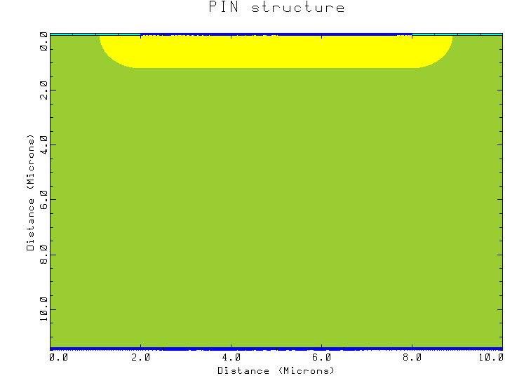
代码 1 PIN 结构
title PIN structure
assign name=pwell n.value=1e17
assign name=ndrift n.value=2.5e15
assign name=Dpsd n.value=0.2
assign name=Dpwell n.value=1.2
assign name=Ddrift n.value=10
assign name=Dsub n.value=0.2
assign name=depth n.value=@Dpwell+@Ddrift+@Dsub
assign name=wide n.value=10
assign name=Wpwell n.value=6
mesh smooth.k=1
x.mesh width=2 h1=0.05
x.mesh width=@Wpwell h1=0.05 h2=0.05 h3=0.5
x.mesh width=2 h1=0.05
y.mesh n=1 L=-0.1
y.mesh n=5 L=0
y.mesh depth=@Dpsd h1=0.04 h2=0.01
y.mesh depth=@Dpwell-@Dpsd h1=0.01 h2=0.05
y.mesh depth=@Ddrift h1=0.05 h2=0.1 h3=1.5
y.mesh depth=@Dsub h1=0.1
y.mesh depth=0.1 h1=0.05
region name=si y.min=0 silicon
region name=fox y.max=0 oxide
electrode name=anode x.min=2 x.max=@wide-2 y.min=-0.1 y.max=0
electrode name=cathode y.min=@depth
$$ ndrift $$
profile reg=si uniform n.type n.peak=@ndrift
$$ pwell/psd $$
profile reg=si p.type n.peak=@pwell x.min=2 x.max=@wide-2 y.junction=@Dpwell xy.ratio=0.75
profile reg=si p.type n.peak=5e19 x.min=2 x.max=@wide-2 y.junction=@Dpsd xy.ratio=0.75
$$ nsub $$
profile reg=si uniform n.type n.peak=5e19 y.min=@depth-@Dsub
regrid doping log ignore=tso ratio=0.5 cos.ang=0.8 smooth.key=1
model consrh auger conmob fldmob bgn
symbolic gummel carrier=0
method iccg damped
solve initial
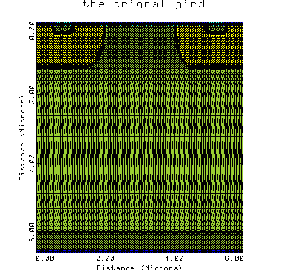
regrid reg=2 poten ratio=1 cos.ang=0.8 max=1 smooth.key=1 out.f=pin.mesh
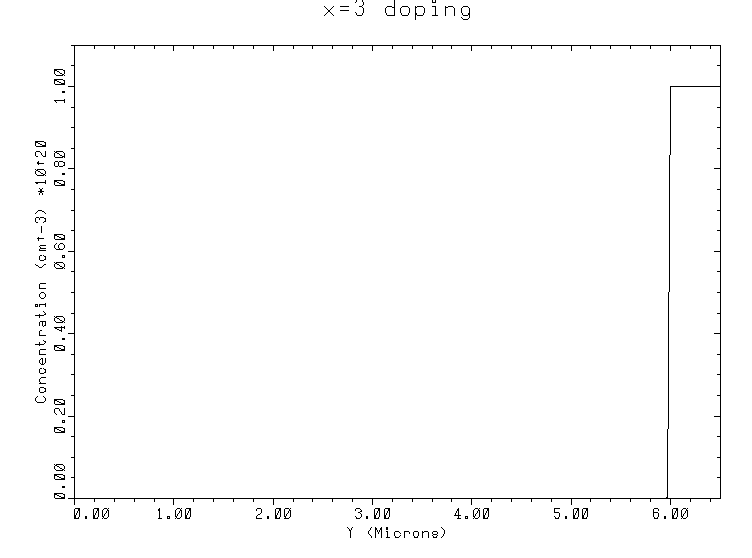
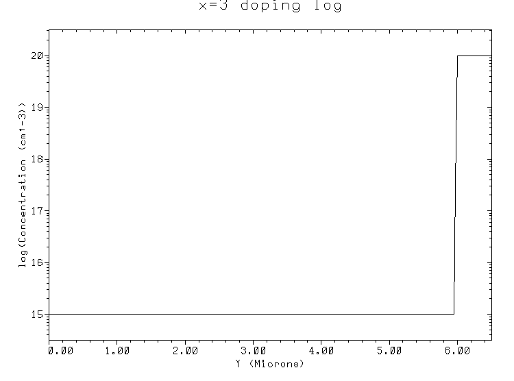
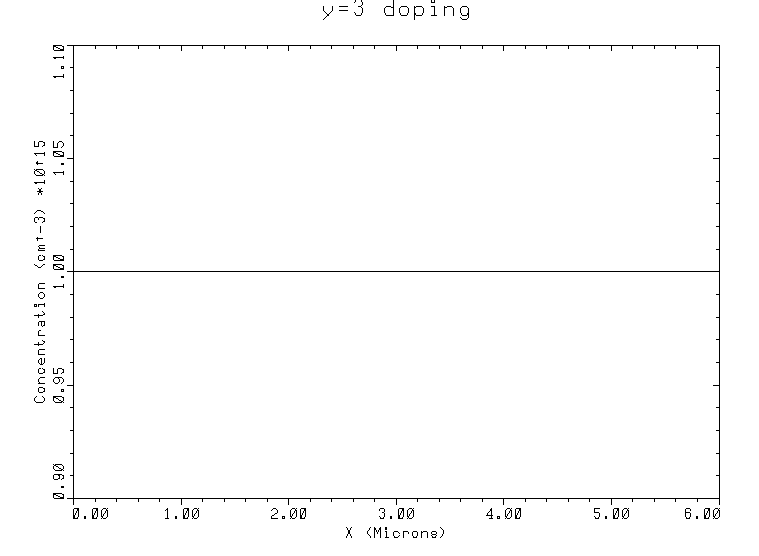
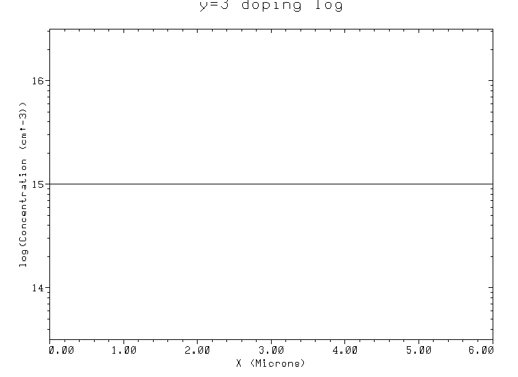
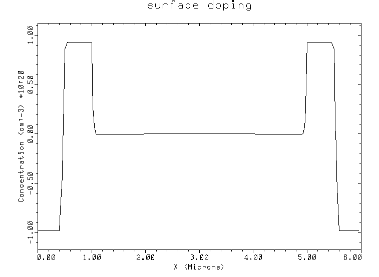
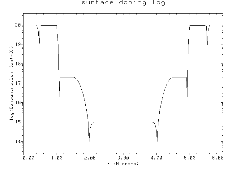
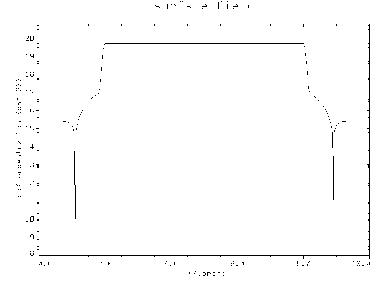
plot.1d doping y.start=0 y.end=0 y.log title="surface field"
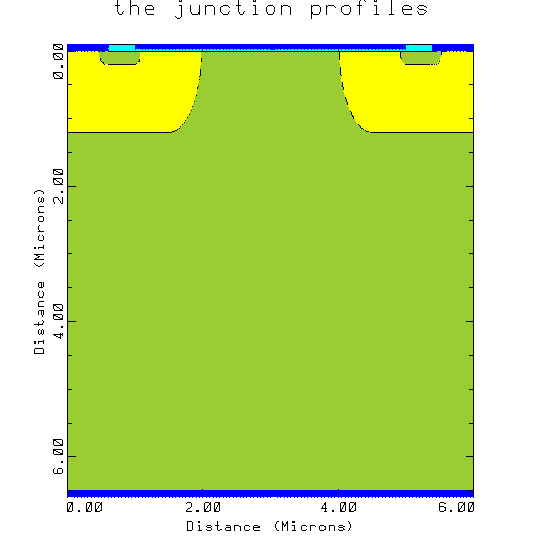
plot.2d bound grid fill
plot.2d bound grid fill
plot.2d bound fill grid scale
plot.2d bound fill
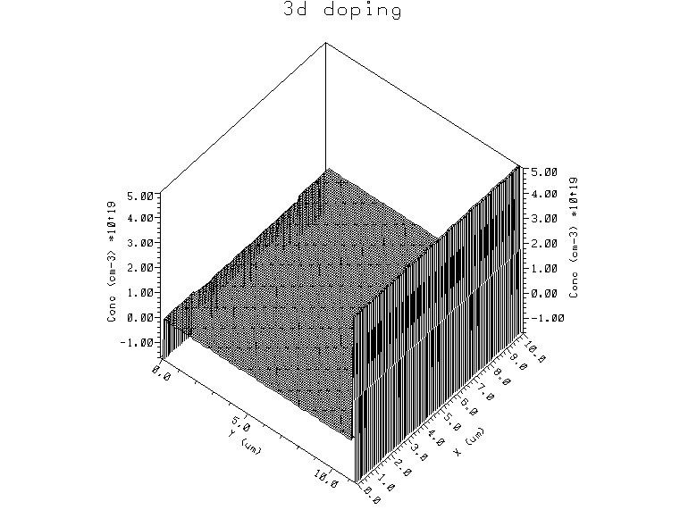
plot.3d doping title="3d doping"
// 定义变量
title PIN structure // 模型标题
assign name=pwell n.value=1e17 // 阱区掺杂浓度
assign name=ndrift n.value=2.5e15 // 漂移区掺杂浓度
assign name=Dpsd n.value=0.2 // PSD区域深度
assign name=Dpwell n.value=1.2 // 阱区深度
assign name=Ddrift n.value=10 // 漂移区深度
assign name=Dsub n.value=0.2 // 衬底区深度
assign name=depth n.value=@Dpwell+@Ddrift+@Dsub // 总深度
assign name=wide n.value=10 // 横向宽度
assign name=Wpwell n.value=6 // 阱区横向宽度
// 生成二维网格
mesh smooth.k=1
x.mesh width=2 h1=0.05 // 源极侧网格
x.mesh width=@Wpwell h1=0.05 h2=0.05 h3=0.5 // 阱区网格
x.mesh width=2 h1=0.05 // 漏极侧网格
y.mesh n=1 L=-0.1 // 顶部空气
y.mesh n=5 L=0 // 氧化物
y.mesh depth=@Dpsd h1=0.04 h2=0.01 // PSD区
y.mesh depth=@Dpwell-@Dpsd h1=0.01 h2=0.05 // 阱区
y.mesh depth=@Ddrift h1=0.05 h2=0.1 h3=1.5 // 漂移区
y.mesh depth=@Dsub h1=0.1 // 衬底区
y.mesh depth=0.1 h1=0.05 // 底部空气
// 定义区域
region name=si y.min=0 silicon // 定义硅区
region name=fox y.max=0 oxide // 定义氧化物区
// 定义电极
electrode name=anode x.min=2 x.max=@wide-2 y.min=-0.1 y.max=0 // 定义阳极
electrode name=cathode y.min=@depth // 定义阴极
// 掺杂剖面
$$ ndrift $$ // 漂移区掺杂
profile reg=si uniform n.type n.peak=@ndrift
$$ pwell/psd $$ // P 阱区和PSD掺杂
profile reg=si p.type n.peak=@pwell x.min=2 x.max=@wide-2 y.junction=@Dpwell xy.ratio=0.75
profile reg=si p.type n.peak=5e19 x.min=2 x.max=@wide-2 y.junction=@Dpsd xy.ratio=0.75
$$ nsub $$ // 衬底区掺杂
profile reg=si uniform n.type n.peak=5e19 y.min=@depth-@Dsub //uniform 为均匀掺杂;n.peak 定义了 n 掺杂的峰值
// 重新生成网格
regrid doping log ignore=tso ratio=0.5 cos.ang=0.8 smooth.key=1
// 设置物理模型
model consrh auger conmob fldmob bgn
symbolic gummel carrier=0
// 设置求解器
method iccg damped
solve initial // 初次求解
// 重新生成更细的网格,regrid 指令在原来的两条线之间加一条;poten
regrid reg=2 poten ratio=1 cos.ang=0.8 max=1 smooth.key=1 out.f=pin.mesh
// 绘制掺杂分布曲线
plot.1d doping y.start=0 y.end=0 y.log title="surface field"
// 绘制二维掺杂分布图
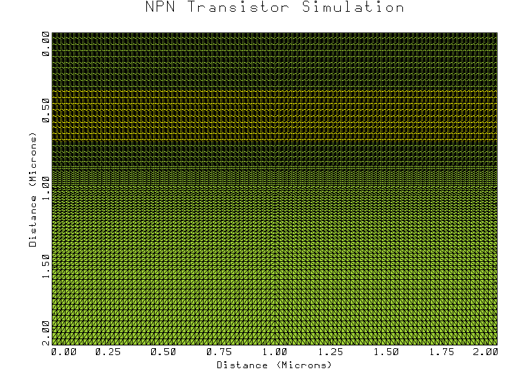
plot.2d bound grid fill
plot.2d bound grid fill
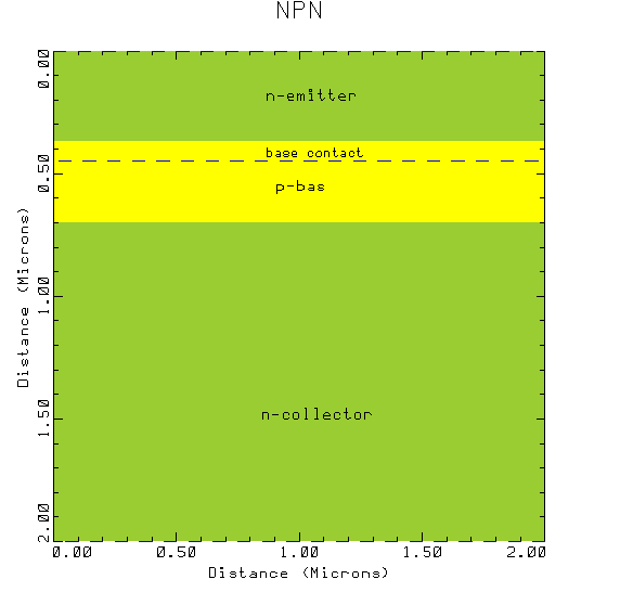
plot.2d bound fill grid scale
plot.2d bound fill
// 绘制三维掺杂分布图
plot.3d doping title="3d doping"仿真使用的三个方程:
Transclude of 空穴连续性方程
Transclude of 电子连续性方程
一维形式的泊松方程
指向原始笔记的链接
为电势; 为电荷密度; 为介电常数。
代码 1 结果

代码 2
$$$$$$ bv characteristic $$$$$$

mesh  in.file=../pin.mesh

MODEL      consrh auger conmob fldmob bgn  srfmob
SYMBOLIC   newton carrier=0
METHODE    damped iccg
SOLVE      initial

MODEL      consrh auger conmob fldmob bgn  impact.i srfmob //impact.i 相当于在连续性方程后面加 Gii
SYMBOLIC   newton carrier=2 block.ma
METHODE    itlimit=20  stack=50
LOG        out.f=bv.log

solve  v(anode)=0

solve electr=cathode v(cathode)=0  vstep=1  nstep=10
solve previous    out.f=bvout2
solve electr=cathode v(cathode)=10  continue c.imax=1e-6 c.vmax=30 c.vstep=1
solve previous    out.f=bvout30
solve electr=cathode v(cathode)=30  continue c.imax=1e-6 c.vmax=50 c.vstep=1
solve previous    out.f=bvout50
solve electr=cathode v(cathode)=50 continue c.imax=1e-6 c.vmax=70 c.vstep=1
solve previous    out.f=bvout70
solve electr=cathode v(anode)=70 continue c.imax=1e-6  c.vmax=90 c.vstep=1
solve previous    out.f=bvout90
solve electr=cathode v(cathode)=100 continue c.imax=1e-6 c.vmax=120 c.vstep=1
solve previous    out.f=bvout120
solve electr=cathode v(cathode)=120  continue c.imax=1e-6 c.vmax=140 c.vstep=1
solve previous    out.f=bvout140
solve electr=cathode v(cathode)=140  continue c.imax=1e-6 c.vmax=160 c.vstep=1
solve previous    out.f=bvout160


$plot.1d  in.file=bv.log y.axis=i(anode)  x.axis=v(anoded) y.log  points  line=1 color=2
+        title="sbr ia vs. va"

solve previous out.f=bvout
extract ion
Lab 2
实验一
实验二
Lab 3 Power Mosfet